• Introduction
• Introduction
• Data-driven research
• Data literacy
• Introducing data
• Types of spending data
• Reference data
• Machine-readable and useable data
• Working with data
• The data processing pipeline
• Getting data
• Cleaning data
• Analysis
• Presentation and engagement
• Framing: topic, objective, audience
• Engaging the public online
• Case study: BudgIT
• Working with others
• Why collaborate?
• Using technology in your work
• Countering arguments against publishing data
• Appendices
• About this book
• Privacy guide
• Resources
• Glossary

Introducing data

In the previous section of the Handbook, you learned about the data-driven research workflow. Now you're probably eager to start answering the big questions about spending using data.

But what do we mean by "spending data", anyway? Is spending data the only kind of data you need in order to investigate spending? And what's the difference between "data" and other ways of presenting information?

This section of the Handbook answers these important questions by explaining the ins and outs of spending data itself. It contains the following chapters:

• Types of spending data. The difference between budgets and proper spending data, and the different kinds of investigations that each is useful for.
• Reference data. Other kinds of datasets that are useful for specific kinds of investigations.
• Machine-readable and useable data. What makes an informative file "data", and what you should ask for when requesting data from governments or other sources.

What is data?

Data is all around us. But what exactly is it?

Data is a value assigned to a thing. Consider, for example, the balls in the picture below.

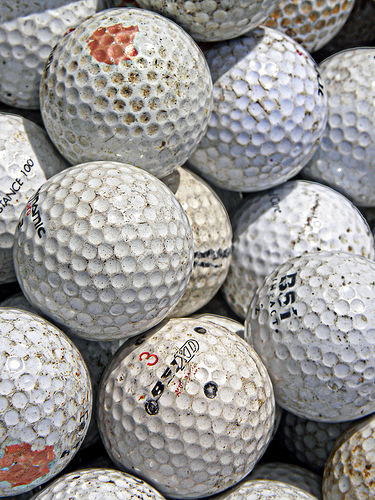
What can we say about these? They're golf balls, right? So one of the first data points we have is that they are used for golf. Golf is a category of sport, so this helps us to put the ball in a taxonomy. But there is more to them. We have their colour (white) and their condition (used). They all have a size, there is a certain number of them, they each have some monetary value, and so on.

Even unremarkable objects have a lot of data attached to them. You do, too: you have a name (most people have given and family names), a date of birth, weight, height, nationality etc. All these things are data.

In the example above, we can already see that there are different types of data. The two major categories are qualitative and quantitative data.

Qualitative data is everything that refers to the quality of something: a description of colours, the texture and feel of an object, a description of experiences, and an interview are all qualitative data.

Quantitative data is data that refers to a number, e.g. the number of golf balls, the size, the price, a score on a test, etc.

There are also other categories that you will most likely encounter:

Categorical data puts the item you are describing into a category. In our example, the condition "used" would be categorical (with other categories such as "new", "used", "broken", etc.)

Discrete data is numerical data that has gaps in it, e.g. the count of golf balls. There can only be whole numbers of golf ball (there is no such thing as 0.3 golf balls). Other examples are scores in tests (where you might receive, for example, 7/10) or shoe sizes.

Continuous data is numerical data with a continuous range. The size of the golfballs, for example, can be any value (e.q. 10.53mm or 10.54mm but also 10.536mm), as can the size of your foot (as opposed to your shoe size, which is discrete).

Unstructured vs. Structured data

“quantity”, “color”, “condition”, “item”, “category”, “diameter (mm)”, “price per unit (AUD)”
5,”white”,”used”,”ball”,”golf”,43,0.5